How to Build an RFM Score Using Python
DIY RFM: A Step-By-Step Guide
What even is RFM? A pirate’s favorite radio station? The secret level of sleep that’s even deeper than REM sleep? No, it stands for Recency Frequency Monetary, and it’s a simple tool that organizations can use to identify strong prospects. After reading this post, I hope you’ll agree with me that it might as well stand for Really Fun Metric! Let’s break down the ingredients:
R is for Recency: When was a prospect’s last gift? Prospects who have given more recently are generally better targets because they are more likely to give again. As we saw in this post, the longer it’s been since a prospect’s last gift, the less likely they are to give again.
F is for Frequency: How many gifts has a prospect made? Prospects who make many gifts are telling you that they are invested in your mission and want you to succeed. Also frequent giving, even at small levels, is a strong indicator for planned gifts.
M is for Monetary: How much has a prospect given in total over its lifetime? You could also measure this as what a prospect’s single largest gift has been. Using total giving illustrates a prospect’s lifetime value to the organization, while using the largest single gift helps an organization understand what the prospect’s capacity might be and may be a better route if you want to focus on major giving. I’ll be using the total giving version, but use what works best for you; the information in this post will work just the same regardless of which one you choose.
To develop an RFM score, you first assign values to each of the ingredients, and then combine these values in some way to identify your best prospects overall. Now that we understand what an RFM score is, we can explore why you should want one. RFM is a very simple metric, particularly compared to metrics produced by AI and machine learning models, but from this simplicity comes the true value of RFM.
- It only has 3 ingredients, which makes it more understandable to a broader audience than algorithms like a Random Forest or Gradient Descent.
- It’s based on solely on your existing data, meaning you don’t have to worry if a third-party’s input is credible or reliable like you might with gift capacities, for example.
- The scores are built on the actual real-world behaviors of your donors. Therefore, your scores are going to be specific to your donors at your organization, and not generalized from data across the country or industry.
Not quite sold on calling it Really Fun Metric yet? Fair enough. I’ll check back after you see how easy it is to set up.
Why Use Python?
RFM is so simple that you can calculate it only using Microsoft Excel. However, I like to use the Python programming language with the pandas library over Excel for two reasons: (1) it sounds cooler to say that you work with pandas and pythons than spreadsheets, and (2) Python and pandas are much faster and more flexible than Excel. How many times have you been working with a large data set and Excel freezes and displays the dreaded “Microsoft Excel Not Responding” message? I’ve had to force-quit my fair share of Excel sessions and lost time and data because it froze before I could click “Save”. With Python, you can manipulate large amounts of data without the same level of worry about freezing or losing your work. In fact, the script that we’re about to go through can take a file with over 500,000 rows of gifts, aggregate those gifts for each prospect, and calculate the RFM scores for each prospect in under 2 minutes. Processing files of that size that quickly in Excel is pretty much impossible.
Additionally, Excel has a size limit of just over 1 million rows while pandas does not have a limit. Granted, 1 million rows is a lot, but some projects involve a couple million rows, and staying in Excel means you’re forced to split it up into multiple worksheets and workbooks. The last main benefit I’ll offer is that you only have to write the script once, and then can click “run” whenever you want new scores in the future. You can quickly update your data every six months, every quarter, or heck, even every day if you’ve just got to have those fresh-squeezed RFM scores first thing each morning. With Excel you would need to string together some complex macros in VBA to make this a repeatable process, and even then you still have the size and speed limitations.
Case Study: Wossamotta University
Let’s jump in and go step by step on how to calculate RFM scores using Python for our friends at Wossamotta University* (Wossamotta U for short). A word of warning: This isn’t an instruction guide for learning Python or the pandas library, but rather how to use Python and pandas to develop RFM scores, so I’m assuming that you have some basic knowledge coming in. However, if you are brand new to Python, here’s a great resource that I found really helpful when starting out. Python is a very beginner-friendly language, so I have no doubt that you’ll be able to get up and running in no time, and there’s a lot more you can do with it beyond calculating RFM scores.
*Wossamotta U is a fictional university whose most notable alumni are Rocky the Flying Squirrel and Bullwinkle J. Moose. As such, the data shown here is fictional, randomly generated and modeled to simulate real-world giving data.
Step 0: Get your Data and Coding Environment Ready
Before we actually start writing our program in Step 1, we need to make sure we have all our tools ready.
- We start by importing the pandas library which will allow us to read and manipulate spreadsheet-style data like .xlsx or .csv files.
- Next, we need to load in our data. Our data file is a simple list of gift records that only requires three basic fields: Prospect IDs, Gift Dates, and Gift Amounts. My file also has a Gift ID field, but it’s not necessary.
- We load our file as a pandas DataFrame (basically a table) using the .read_excel( ) function and we can take a peek at the first five rows of our data file using the .head( ) function.

Step 1: Group Gifts by Prospect and Calculate the Basic Ingredients of RFM
Now we’re ready. Our first step is going to be converting our list of gift records, into a list of prospects, and calculating each ingredient of RFM:
- R Ingredient: When was their most recent gift?
- F Ingredient: How many gifts have they made in their lifetime?
- M Ingredient: How much is their total lifetime giving?
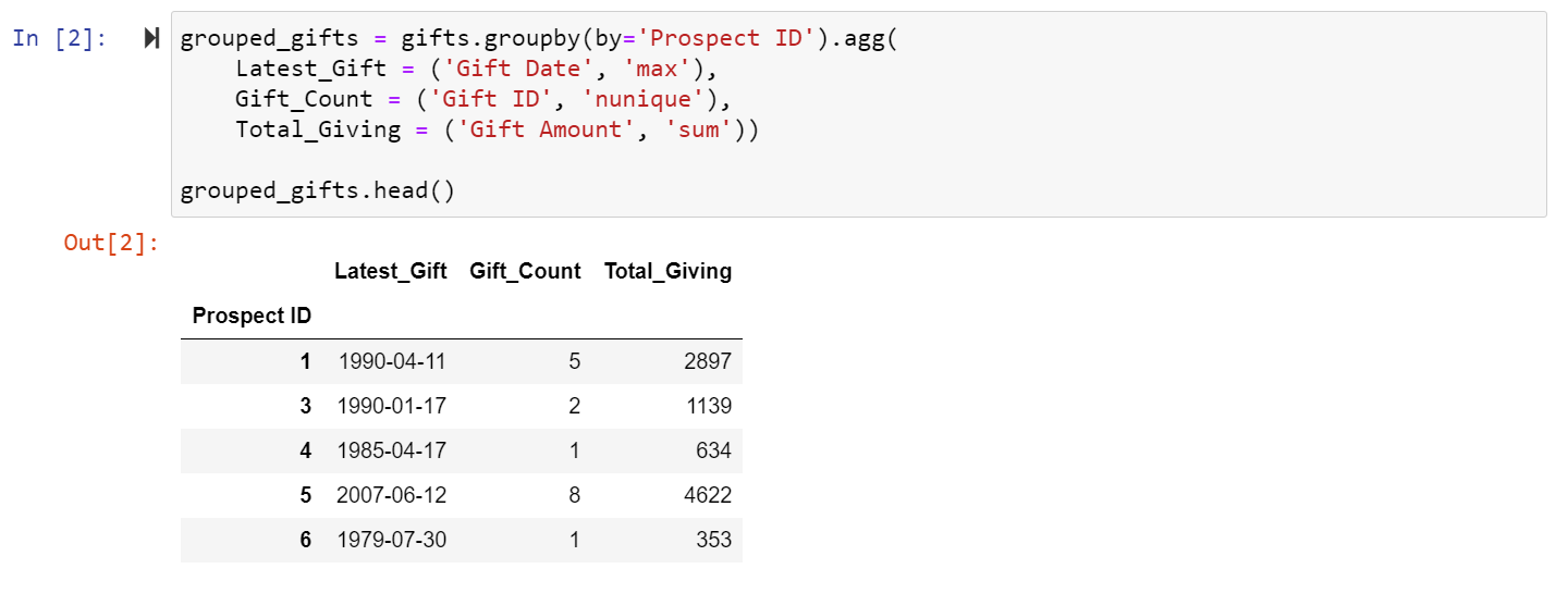
We can accomplish this pretty easily by using the .groupby( ) and .agg( ) functions. Again, we’ll use the .head( ) function to see the first five rows. Instead of gift records, now each row shows us a prospect and their RFM ingredients.
Step 2: Calculate and Assign RFM Values to Each Prospect
We have the basic ingredients for RFM for each prospect. Now, we have to compare all the prospects against one another and assign a value of 1-5 for each ingredient based on how a prospect compares to the rest of the population. Using a scale of 1-5 is somewhat arbitrary, you could do 1-4 or 1-10, but using 1-5 allows us to split the data into quintiles (20% chunks). The bottom 20% will be assigned a value of 1, the next 20% chunk will be assigned a value of 2, and so on from there until the top 20% are assigned a value of 5. Higher values mean that a prospect has given more recently, made more gifts, and/or given more money when compared to their peers; a prospect with all 5s is one of your strongest prospects.
To figure out what each prospect’s values are, we first calculate what percentile each of their ingredients fall into compared to the whole group. This is easily done in one line with the pandas function .rank(pct=True).

Let’s interpret our results by looking at the first prospect on our list. When we found their basic ingredients, we saw they last gave on 1990-04-11, they had made 5 gifts to the university, and those 5 gifts totaled $2,897. With the percentile data, we can see that their latest gift is around the 13th percentile among all latest gifts. This means that 87% of our prospects have made a gift more recently than this person. Their gift count is only in the 2nd percentile, meaning that 98% of our prospects have made more gifts than this person. And lastly their total giving is in roughly the 17th percentile of all total giving amounts, so 83% of our prospects have given more money to the university. Initially, this prospect doesn’t look very strong, but we can make that easier to see by converting their percentiles into values of 1-5.
Unfortunately, Python and pandas don’t have a built-in RFM function to assign these values automatically, but we can easily create our own function using the def function_name( ) command and we’ll name it get_rfm_values so that it clearly shows what it’s doing. We’ll make it so our function will take in a percentile, and if that percentile is between 0 and 0.2 (0 – 20th percentiles), we assign a value of 1. If the percentile is between 0.2 and 0.4 (21st – 40th percentiles), we assign a value of 2. This process repeats until we assign a value of 5 to percentiles between 0.8 and 1.0 (80th – 100th percentiles). Then we can use the pandas function .applymap( ) to run every percentile in our entire table through our self-created get_rfm_values( ) function. After that, we rename the columns to represent that we are now showing the R, F, and M values for each prospect.
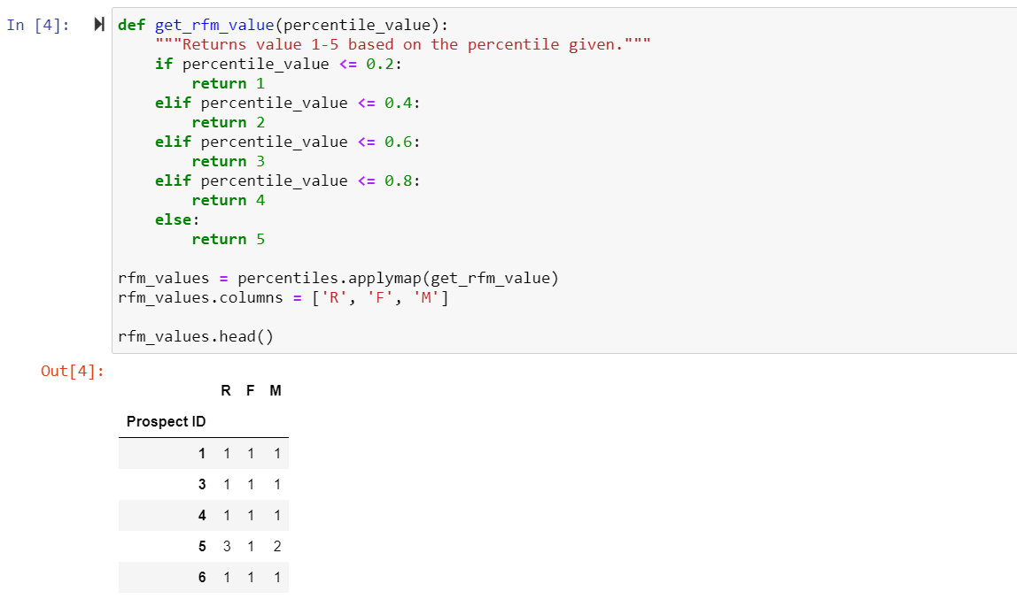
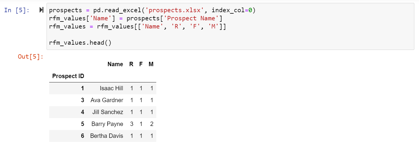
Right now, our table is all numbers and isn’t very easy to read! Let’s bring in our prospects’ names to give all these numbers a little more context and clarity. First we’ll have to load in our prospect data file, and then we can add in the Prospect Name that corresponds to each Prospect ID on our RFM table. Lastly, we’ll reorder the columns so that the name comes before the R, F, and M values.
Step 3: Choose an Approach to Return Overall RFM Scores
We’re nearly done! This is essentially our last step, but it’s the most important. Now is when we decide what to do with these RFM values of 1-5. Here are three potential options, each with their own strengths and weaknesses:
- Base Values Approach
- Simple Aggregation Approach
- Weighted Aggregation Approach
Base Values Approach
The Base Values Approach is very simple, we don’t need to do anything other than a little formatting and concatenation. In Python, we can utilize the .apply( ) and lambda functions to take our three columns of integer values and convert them into a single string formatted as “R-F-M”. Then we can add the results to our table and display the first five rows.
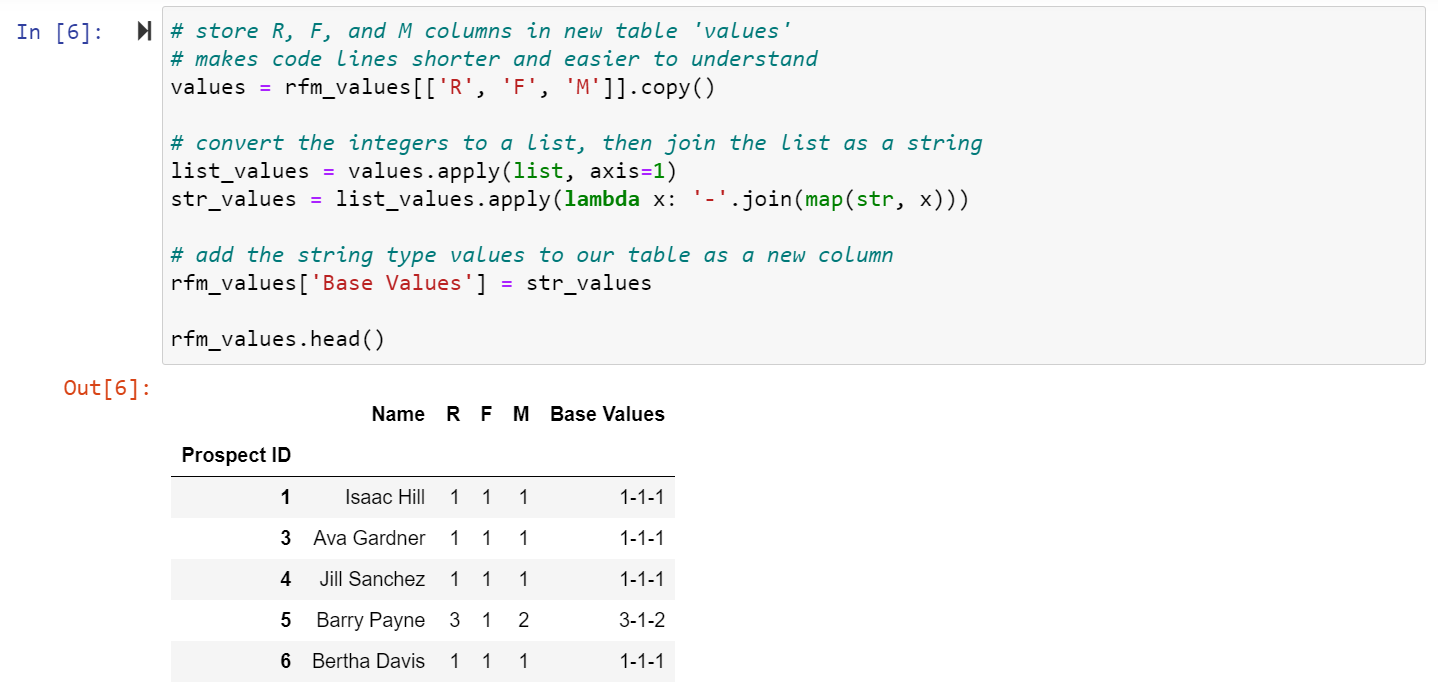
This is the simplest approach to take, and is just a formatted display of the R, F, and M values. Despite being the easiest to produce, the results are probably the most difficult to interpret. Anyone who wants to utilize these results needs to know that the three digits correspond to Recency, Frequency, and Monetary (in that order) and needs to remember what each of those terms mean. They’ll also need to take into consideration if any one of the values is more important than the others and be able to know how that might change a prospect’s priority. That’s a lot to ask of anyone, and it would be easier if we could boil it down to a single number, enter Simple Aggregation.
Simple Aggregation Approach
The Simple Aggregation Approach is just as easy as the Base Values Approach. All we have to do is add up R + F + M, to end up with a single score ranging from 3 (1 + 1 + 1) to 15 (5 + 5 + 5). This is very easy to do in pandas even for hundreds of thousands of prospects. We can use the .apply( ) function to calculate the sum of the three values for each prospect, add the results as a new column to our table, and show the first five rows to see what we get.

The advantage Simple Aggregation has over Base Values is that the results are much easier to interpret. Anyone can use these scores to decide which prospect is stronger than another. However, in this simplification, the nuance of how the score was calculated is lost. Here’s an example of why that’s important to know.
A prospect with the values 1-5-5 would have a Simple Aggregation score of 11. But a prospect with values of 5-5-1 would also get a score of 11. The first prospect’s R value is 1, and they likely haven’t made a gift in decades, but their F and M values tell us that in the past, they gave often and at large amounts. The second prospect’s R and F values tell us that they are one of the most recent donors, who has been giving often. But their M value of 1 shows that they have only been making small gifts. These two prospects clearly do not have similar giving behaviors, but the Simple Aggregation Approach gives them identical scores. We need a way to prioritize which of them is the better prospect overall, and we can accomplish this with the Weighted Aggregation method.
Weighted Aggregation Approach
The Weighted Aggregation Approach is the most complex to perform, however it solves both problems with the Base Values and Simple Aggregation approaches. Weighted Aggregation will give us an easy-to-interpret score while still taking into consideration the nuances of each value and the different importance, or weight, an organization places on R, F, and M. At Wossamotta U for example, they feel that a prospect’s M value (total giving) is most important and should account for 50% of a prospect’s overall RFM score. The R values are second in importance to the university, and should account for 30% of the overall score, while the F values make up the remaining 20% of the overall score. Wossamotta U highly values prospects who have given large amounts of money, and those who have done so fairly recently. They don’t care as much about how many gifts the prospect has made. If you decide that all the values are equally important, you could just stick with the Simple Aggregation Approach and call it a day!
Okay, we know how Wossamotta U feels about each of the R, F, and M values. What next? I recommend scaling the values so that a score of 100 represents the best possible score. It doesn’t have to be 100, you could decide you want the best possible score to be 420, you little jokester! But most everyone understands scores out of 100, so that’s why I recommend it. In order to convert our three values into a single number out of 100, we’ll need to do a little bit of math.
Anxiety and Dread have entered the chat…
Don’t leave just yet! I promise it will only be a little bit of basic math, and with the knowledge instilled in me by my 8th grade pre-algebra teacher, Mr. Rauhauser, we’ll get through this together. The best possible set of RFM values is 5-5-5, so we’re trying to figure out a way to start with three 5s and end up with 100. If we were to just add them together (the Simple Aggregation Approach), we’d only get to 15. So before we add them together, we have to scale, or multiply, our original values of 5s into bigger values that will add up to 100. What we need multiply our values by depends on the weight of each value as determined by the organization.
We’ll start with R. Wossamotta U feels that the R value should account for 30% of a prospect’s overall score. If the highest score we want is 100 points, our highest possible R value would be 30 (30% of 100). So, we need to scale our R values by whatever turns the original highest score of 5 into the new highest score of 30. According to my old multiplication tables, that means we multiply R by 6 and the original values of [1, 2, 3, 4, 5] now become [6, 12, 18, 24, 30]. Still with me? Good. Let’s do the same process for the other two components of RFM.
The F value should account for 20% of a prospect’s overall score. For the highest score of 100, this means that the highest possible F value is 20 (20% of 100). We need to scale our F values by whatever turns the original highest score of 5 into the new highest score of 20. That means we multiply F by 4 and the original F values of [1, 2, 3, 4, 5] now become [4, 8, 12, 16, 20].
Finally, the M value needs to account for 50% of a prospect’s overall score. For the highest score of 100, this means that the highest possible M value is 50 (50% of 100). We need to scale our M values by whatever turns the original highest score of 5 into the new highest score of 50. That means we multiply M by 10 and the original M values of [1, 2, 3, 4, 5] now become [10, 20, 30, 40, 50].
That was a lot to take in, but hopefully you can see that after we’ve scaled everything up based on the weights, our original best RFM values of 5-5-5 now have become 30-20-50. Now we can add those together to get 100. We did it, I’m so proud of you! Luckily for us, now that we’ve figured out what we need to scale by, implementing the scaling in Python is super quick. I have created a quick little function called get_weighted_agg( ) and can use the .apply( ) function to take our three values for each prospect, scale them up by the appropriate amounts (6x, 4x, and 10x), add those scaled values together, and then add that final score as a new column to our table.
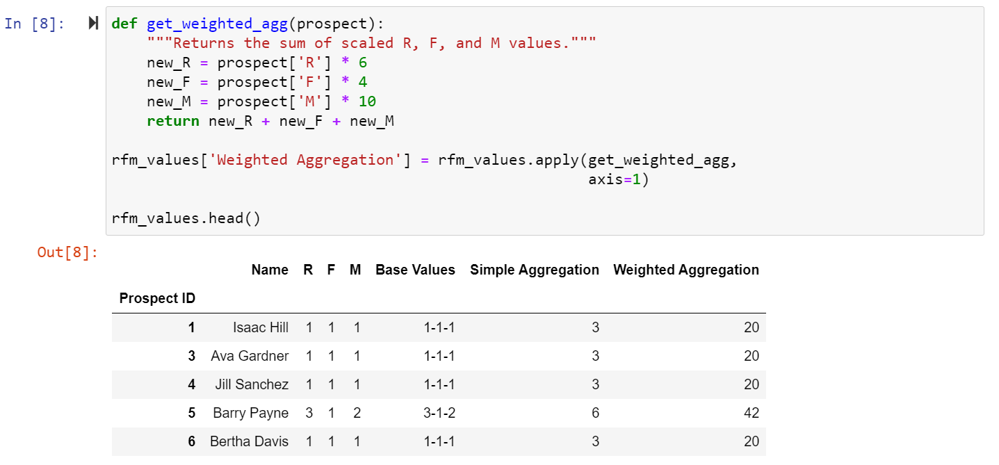
Weighted Aggregation is the best approach of these 3. Not only is the final score a single number out of 100, but the process ensures that we are valuing giving behaviors appropriately. Remember those two prospects from the example in Simple Aggregation? They had RFM values of 1-5-5 and 5-5-1, and the Simple Aggregation Approach determined they were equally valuable prospects. Following Weighted Aggregation, the first prospect would have values of 6-20-50 for a score of 76 while the second prospect would have values of 30-20-10 for a score of 60. Based on how Wossamotta U thinks about Recency, Frequency, and Monetary values, the first prospect is a stronger prospect and should be prioritized first.
Comparing the Approaches
Below is the data for three of Wossamotta U’s prospects: Boris Badenov, Natasha Fatale, and Dudley Do-Right. University leadership has asked us, “Which prospect is best? Who should we prioritize and focus our efforts on?” Their most recent gifts have all been made within six months of each other. Their total gift counts are all pretty close, and they’ve all given right around $50,000. It would be very difficult for us to try and prioritize between them based just on these data points, so we’ll calculate RFM scores using each of the three approaches and compare the results.
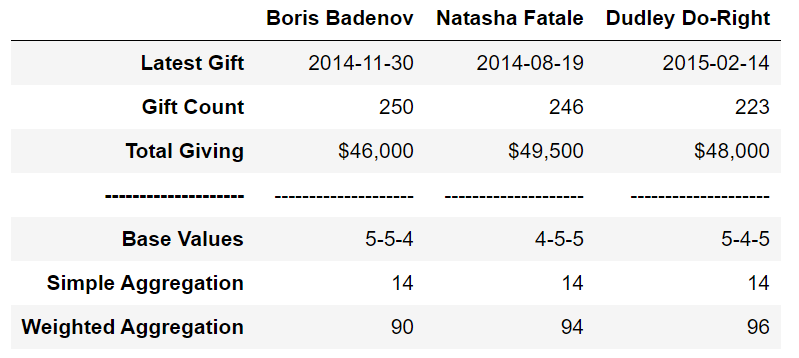
The Base Values Approach gives us the down and dirty details on each prospect and how they scored across all three values. While it is possible for us to pick the best prospect from these results, it wouldn’t be very easy to explain how we arrived at that decision.
The Simple Aggregation Approach gives us results that are easy to understand and explain but are not very helpful. Because all three prospects have the same combination of RFM values, they all receive the same score which makes prioritizing one over the others impossible.
The results from the Weighted Aggregation Approach give us the best of both worlds; we have the simplicity of a single number score like Simple Aggregation but have kept the details found in Base Values. Through Weighted Aggregation, we’re able to answer that Dudley Do-Right is the best prospect of these three based on RFM. Without taking the Weighted Aggregation Approach, I doubt that our choice would be that easy, because Dudley has lowest gift count and second-lowest total giving. Prioritizing between three prospects is not exactly a real-world scenario, but when we extend this approach to thousands of prospects, we can easily distill that population down to a manageable group to prioritize.
Step 4: Export Final RFM Scores and Celebrate
All that’s left to do now, is export our final RFM scores into a file that we can easily share with the database team or whoever needs it. We can use the pandas .loc[ ] method to isolate just the columns we want from our table, then rename those columns for clarity, and finally export our scores to an Excel file with the .to_excel( ) function.

And just like that, we’ve written a computer program that opens a file containing gift records, calculates the RFM scores for all of our prospects, and then produces a new file with those scores. You’re basically a professional computer programmer now. Congratulations!
Incorporating RFM Scores
Try as we might, we won’t ever develop a single score that can perfectly encapsulate everything there is to know about a prospect. RFM is a good start, but I would advise our friends at Wossamotta U to incorporate RFM with other metrics or scores they already have, like gift capacity. I might recommend that they filter their prospects to only look at those with RFM scores of at least 95, and then sort by gift capacity to further segment and prioritize the prospects for their fundraisers. Or the reverse approach would work to filter for only certain gift capacities, and then focus on those with the highest RFM scores.
Another way to incorporate RFM is to strategically target a smaller group for direct-mail solicitations. Lapsed donors are very hard to bring back and soliciting all of them is not a cost-efficient strategy. However, if Wossamotta U focused on the lapsed donors with the highest RFM scores, they would be able to lower their mailing costs while targeting the prospects who are more likely to come back based on their giving behaviors. They would be spending less, and would likely be recapturing lapsed donors at higher rates than before.
Wrapping Up
Have I convinced you that RFM is a Really Fun Metric? If not, you at least came away from this with a solid dad joke about it being a pirate’s favorite radio station. Trust me, that will kill at any fundraising conference. But in all seriousness, hopefully you were able take something away from this. If you already have an RFM score provided by a vendor, maybe now you feel comfortable on developing your own and reallocating that budget elsewhere. Or maybe this brought up some other ideas of how you could use Python and pandas to develop a different score that you don’t already have. Or maybe you just chuckled once or twice and were briefly distracted from the dumpster fire that has been 2020. Whatever you got out of this, thank you for reading it.